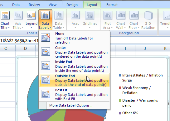
45 add data labels to the best fit position
Adding Data Labels to Your Chart (Microsoft Excel) - ExcelTips (ribbon) Select the position that best fits where you want your labels to appear. To add data labels in Excel 2013 or later versions, follow these steps: Activate the chart by clicking on it, if necessary. Make sure the Design tab of the ribbon is displayed. (This will appear when the chart is selected.) Click the Add Chart Element drop-down list. Marketing, Automation & Email Platform | Mailchimp Mailchimp is the #1 email marketing and automation brand based on competitor brands' publicly available data on worldwide numbers of customers in 2021 / 2022. Generate up to 4X more orders with Customer Journey Builder automations based on orders generated through user's connected stores with automations versus when they used bulk emails.
Fit Chart Labels Perfectly in Reporting Services using Two Powerful ... Make the labels smaller. Move or remove the labels. Option #1 gets ruled out frequently for information-dense layouts like dashboards. Option #2 can only be used to a point; fonts become too difficult to read below 6pt (even 7pt font can be taxing to the eyes). Option #3 - angled/staggered/omitted labels - simply may not meet our needs.
Add data labels to the best fit position
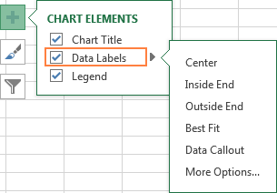
How to add or move data labels in Excel chart? - ExtendOffice 2. Then click the Chart Elements, and check Data Labels, then you can click the arrow to choose an option about the data labels in the sub menu. See screenshot: In Excel 2010 or 2007. 1. click on the chart to show the Layout tab in the Chart Tools group. See screenshot: 2. Then click Data Labels, and select one type of data labels as you need ... Office: Display Data Labels in a Pie Chart - Tech-Recipes: A Cookbook ... 1. Launch PowerPoint, and open the document that you want to edit. 2. If you have not inserted a chart yet, go to the Insert tab on the ribbon, and click the Chart option. 3. In the Chart window, choose the Pie chart option from the list on the left. Next, choose the type of pie chart you want on the right side. 4. How to add trendline in Excel chart - Ablebits.com On the Format Trendline Label pane that appears, go to the Label Options tab. In the Category drop-down list, select Number. In the Decimal places box, type the number of decimal places you want to show (up to 30) and press Enter to update the equation in the chart. How to find the slope of a trendline in Excel
Add data labels to the best fit position. Customize Axes and Axis Labels in Graphs - JMP Get Your Data into JMP. Copy and Paste Data into a Data Table. Import Data into a Data Table. Enter Data in a Data Table. Transfer Data from Excel to JMP. Work with Data Tables. Edit Data in a Data Table. Select, Deselect, and Find Values in a Data Table. View or Change Column Information in a Data Table. VBA Bestfit position for datalabels on line chart - Stack Overflow "Best fit" is a setting unique to pie chart data labels. You have the option of positioning a line chart's data labels centered (directly on a point), as well as above, below, left of, and right of the point. You can also position the data label anywhere by changing the .left and .top properties of the label. Excel VBA Code for data label position | MrExcel Message Board If you select 'Format Data Labels' using the right-click context menu on a label, the properties pane on the right hand side only has 'Centre', 'Inside End' and 'Inside Base' for column charts (for example). As I want to move a column label above the column I suspect I'm going to have to move it to an absolute position . The Best Pillow for Your Sleep Position - Consumer Reports Sep 14, 2022 · The purpose of a pillow is pretty simple: to keep your head and neck aligned while you sleep. If only shopping for pillows were as straightforward. Store shelves and catalogs are stuffed with ...
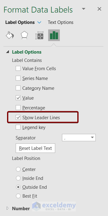
Series.DataLabels method (Excel) | Microsoft Learn This example sets the data labels for series one on Chart1 to show their key, assuming that their values are visible when the example runs. With Charts("Chart1").SeriesCollection(1) .HasDataLabels = True With .DataLabels .ShowLegendKey = True .Type = xlValue End With End With Support and feedback Custom Excel Chart Label Positions • My Online Training Hub Custom Excel Chart Label Positions - Setup. The source data table has an extra column for the 'Label' which calculates the maximum of the Actual and Target: The formatting of the Label series is set to 'No fill' and 'No line' making it invisible in the chart, hence the name 'ghost series': The Label Series uses the 'Value ... Excel Charts: Dynamic Label positioning of line series - XelPlus Select your chart and go to the Format tab, click on the drop-down menu at the upper left-hand portion and select Series "Actual". Go to Layout tab, select Data Labels > Right. Right mouse click on the data label displayed on the chart. Select Format Data Labels. Under the Label Options, show the Series Name and untick the Value. The Ultimate Guide to Data Labeling for Machine Learning - CloudFactory In machine learning, if you have labeled data, that means your data is marked up, or annotated, to show the target, which is the answer you want your machine learning model to predict. In general, data labeling can refer to tasks that include data tagging, annotation, classification, moderation, transcription, or processing.
NCES Kids' Zone Test Your Knowledge - National Center for ... The NCES Kids' Zone provides information to help you learn about schools; decide on a college; find a public library; engage in several games, quizzes and skill building about math, probability, graphing, and mathematicians; and to learn many interesting facts about education. Interactivate: Activities Enter a set of data points and a function or multiple functions, then manipulate those functions to fit those points. Manipulate the function on a coordinate plane using slider bars. Learn how each constant and coefficient affects the resulting graph. Apply Custom Data Labels to Charted Points - Peltier Tech Click once on a label to select the series of labels. Click again on a label to select just that specific label. Double click on the label to highlight the text of the label, or just click once to insert the cursor into the existing text. Type the text you want to display in the label, and press the Enter key. Data Labels in Power BI - SPGuides Value decimal places: The Value decimal places always should be in Auto mode. Orientation: This option helps in which view you want to see the display units either in Horizontal or in Vertical mode. Position: This option helps to select your position of the data label units. Suppose, you want to view the data units at the inside end or inside the center, then you can directly select the ...
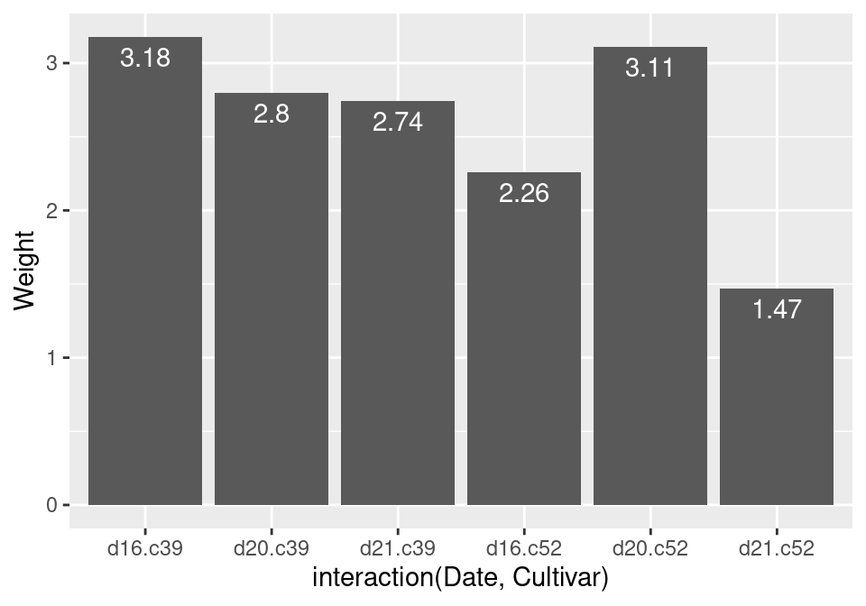
3.9 Adding Labels to a Bar Graph | R Graphics Cookbook, 2nd ...
Matplotlib Bar Chart Labels - Python Guides Firstly, import the important libraries such as matplotlib.pyplot, and numpy. After this, we define data coordinates and labels, and by using arrange () method we find the label locations. Set the width of the bars here we set it to 0.4. By using the ax.bar () method we plot the grouped bar chart.

Dynamically Label Excel Chart Series Lines • My Online ...
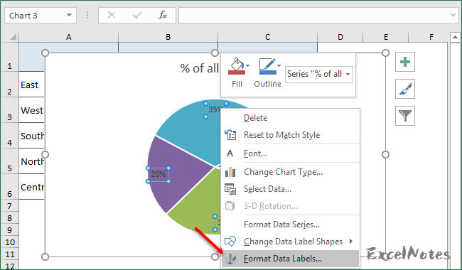
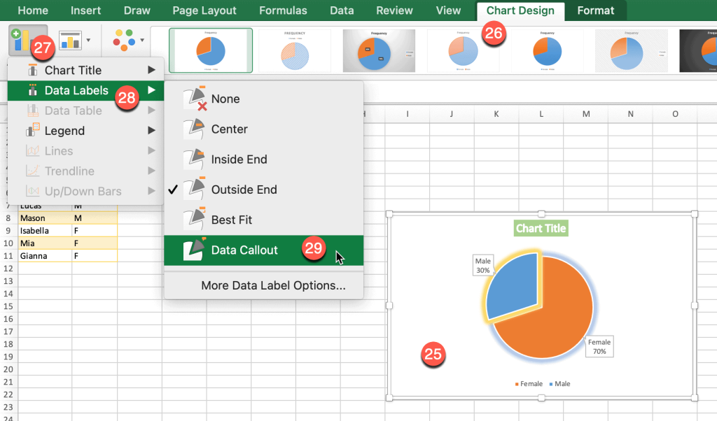
Add or remove data labels in a chart - support.microsoft.com To label one data point, after clicking the series, click that data point. In the upper right corner, next to the chart, click Add Chart Element > Data Labels. To change the location, click the arrow, and choose an option. If you want to show your data label inside a text bubble shape, click Data Callout.
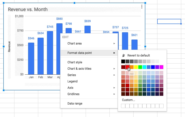
How can I format individual data points in Google Sheets ...
DataLabels Guide - ApexCharts.js In a multi-series or a combo chart, if you don't want to show labels for all the series to avoid jamming up the chart with text, you can do it with the enabledOnSeries property. This property accepts an array in which you have to put the indices of the series you want the data labels to appear. dataLabels: { enabled: true , enabledOnSeries ...
Excel charts: add title, customize chart axis, legend and ...
Page Layouts, Columns and Sections | Confluence Data Center ... Nov 23, 2021 · The layout of your pages can have a big impact on how they're read, and layouts, used well, allow you to position text, images, macros, charts, and much more, to have the best visual impact. There are two ways to modify the layout of a Confluence page: Use page layouts to add sections and columns; Use macros to add sections and columns.

Custom Excel Chart Label Positions • My Online Training Hub
Gui - Syntax & Usage | AutoHotkey Creates and manages windows and controls. Such windows can be used as data entry forms or custom user interfaces. Gui, SubCommand, Value1, Value2, Value3. The SubCommand, Value1, Value2 and Value3 parameters are dependent upon each other and their usage is described below.

how to add data labels into Excel graphs — storytelling with data
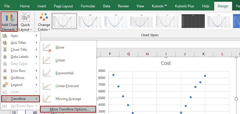
How to add best fit line/curve and formula in Excel? - ExtendOffice There are a few differences to add best fit line or curve and equation between Excel 2007/2010 and 2013. 1. Select the original experiment data in Excel, and then click the Scatter > Scatter on the Insert tab. 2. Select the new added scatter chart, and then click the Trendline > More Trendline Options on the Layout tab. See above screen shot: 3.
How to add and customize chart data labels
How to Customize Your Excel Pivot Chart Data Labels - dummies To add data labels, just select the command that corresponds to the location you want. To remove the labels, select the None command. If you want to specify what Excel should use for the data label, choose the More Data Labels Options command from the Data Labels menu. Excel displays the Format Data Labels pane.
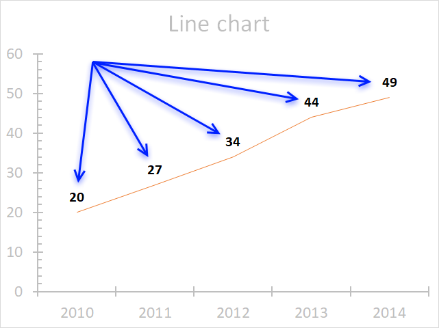
How to Place Labels Directly Through Your Line Graph in ...
Format Data Labels in Excel- Instructions - TeachUcomp, Inc. To do this, click the "Format" tab within the "Chart Tools" contextual tab in the Ribbon. Then select the data labels to format from the "Chart Elements" drop-down in the "Current Selection" button group. Then click the "Format Selection" button that appears below the drop-down menu in the same area.
28 Graphics for communication | R for Data Science
Change the format of data labels in a chart To get there, after adding your data labels, select the data label to format, and then click Chart Elements > Data Labels > More Options. To go to the appropriate area, click one of the four icons ( Fill & Line, Effects, Size & Properties ( Layout & Properties in Outlook or Word), or Label Options) shown here.
Excel 2013: Charts
Format Data Label Options in PowerPoint 2013 for Windows - Indezine Alternatively, select data labels of any data series in your chart and right-click to bring up a contextual menu, as shown in Figure 2, below. From this menu, choose the Format Data Labels option. Figure 2: Format Data Labels option Either of these options opens the Format Data Labels Task Pane, as shown in Figure 3, below.

How to Choose the Best Types of Charts For Your Data - Venngage
Find, label and highlight a certain data point in Excel ... Oct 10, 2018 · Select the Data Labels box and choose where to position the label. By default, Excel shows one numeric value for the label, y value in our case. To display both x and y values, right-click the label, click Format Data Labels…, select the X Value and Y value boxes, and set the Separator of your choosing: Label the data point by name

New charts, formatting, and layout options in Amazon ...
Create Dynamic Chart Data Labels with Slicers - Excel Campus Step 6: Setup the Pivot Table and Slicer. The final step is to make the data labels interactive. We do this with a pivot table and slicer. The source data for the pivot table is the Table on the left side in the image below. This table contains the three options for the different data labels.

How to Add Data Labels to an Excel 2010 Chart - dummies
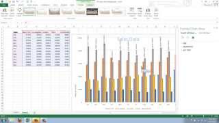
Excel 2010 pie chart data labels in case of "Best Fit" Based on my tested in Excel 2010, the data labels in the "Inside" or "Outside" is based on the data source. If the gap between the data is big, ...

Presenting Data with Charts
Excel 2010 pie chart data labels in case of "Best Fit" Based on my tested in Excel 2010, the data labels in the "Inside" or "Outside" is based on the data source. If the gap between the data is big, the data labels and leader lines is "outside" the chart. And if the gap between the data is small, the data labels and leader lines is "inside" the chart. Regards, George Zhao TechNet Community Support

Add data labels and callouts to charts in Excel 365 ...
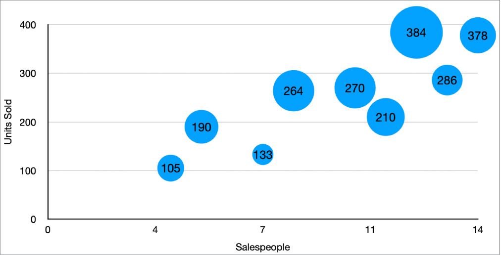
Improve your X Y Scatter Chart with custom data labels - Get Digital Help Press with right mouse button on on a chart dot and press with left mouse button on on "Add Data Labels". Press with right mouse button on on any dot again and press with left mouse button on "Format Data Labels". A new window appears to the right, deselect X and Y Value. Enable "Value from cells". Select cell range D3:D11.
How to Add Totals to Stacked Charts for Readability - Excel ...
12.3. Setting a label — QGIS Documentation documentation 12.3.1.2. Formatting tab . Fig. 12.16 Label settings - Formatting tab . In the Formatting tab, you can:. Use the Type case option to change the capitalization style of the text. You have the possibility to render the text as: No change. All uppercase. All lowercase. Title case: modifies the first letter of each word into capital, and turns the other letters into lower case if the original text ...

How to Represent Data with a Pie of Pie Chart in Your Excel ...
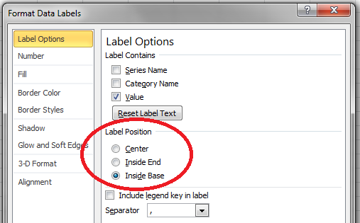
How to Add Data Labels to an Excel 2010 Chart - dummies On the Chart Tools Layout tab, click Data Labels→More Data Label Options. The Format Data Labels dialog box appears. You can use the options on the Label Options, Number, Fill, Border Color, Border Styles, Shadow, Glow and Soft Edges, 3-D Format, and Alignment tabs to customize the appearance and position of the data labels.
python - How to improve the label placement in scatter plot ...
How to add trendline in Excel chart - Ablebits.com On the Format Trendline Label pane that appears, go to the Label Options tab. In the Category drop-down list, select Number. In the Decimal places box, type the number of decimal places you want to show (up to 30) and press Enter to update the equation in the chart. How to find the slope of a trendline in Excel

charts - Excel, giving data labels to only the top/bottom X ...
Office: Display Data Labels in a Pie Chart - Tech-Recipes: A Cookbook ... 1. Launch PowerPoint, and open the document that you want to edit. 2. If you have not inserted a chart yet, go to the Insert tab on the ribbon, and click the Chart option. 3. In the Chart window, choose the Pie chart option from the list on the left. Next, choose the type of pie chart you want on the right side. 4.

New charts, formatting, and layout options in Amazon ...
How to add or move data labels in Excel chart? - ExtendOffice 2. Then click the Chart Elements, and check Data Labels, then you can click the arrow to choose an option about the data labels in the sub menu. See screenshot: In Excel 2010 or 2007. 1. click on the chart to show the Layout tab in the Chart Tools group. See screenshot: 2. Then click Data Labels, and select one type of data labels as you need ...
How-to Make a WSJ Excel Pie Chart with Labels Both Inside and ...

Create Outstanding Pie Charts in Excel | Pryor Learning

Excel: Clustered Column Chart with Percent of Month ...
Add Labels with Lines in an Excel Pie Chart (with Easy Steps)
DataLabels Guide – ApexCharts.js

Change the format of data labels in a chart

How To Make A Pie Chart In Excel Under 60 Seconds

Show, Hide, and Format Mark Labels - Tableau

EXCEL Charts: Column, Bar, Pie and Line

How to Make an Excel Pie Chart
How to Add Data Labels to your Excel Chart in Excel 2013
Change the look of chart text and labels in Numbers on Mac ...
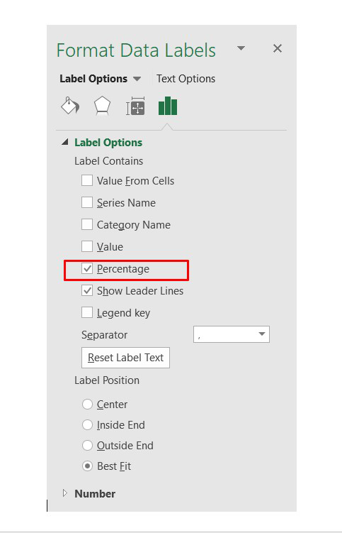
How to Show Percentage in Pie Chart in Excel? - GeeksforGeeks

How to Create a Pie Chart in Excel | Smartsheet
How to add best fit line/curve and formula in Excel?
Excel 2013: Charts

Google Workspace Updates: Get more control over chart data ...
How to Make Pie Chart with Labels both Inside and Outside ...

Hide Zero Values In Data Labels - Excel Titan

Google Workspace Updates: Get more control over chart data ...
How to Add Totals to Stacked Charts for Readability - Excel ...

Format Data Labels in Excel- Instructions - TeachUcomp, Inc.

Office: Display Data Labels in a Pie Chart
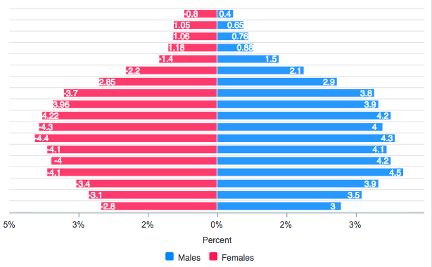
How to ☝️Create a Male/Female Pie Chart in Excel ...
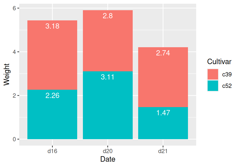
3.9 Adding Labels to a Bar Graph | R Graphics Cookbook, 2nd ...
Post a Comment for "45 add data labels to the best fit position"