38 how to change data labels in excel 2013

› documents › excelHow to change chart axis labels' font color and size in Excel? We can easily change all labels' font color and font size in X axis or Y axis in a chart. Just click to select the axis you will change all labels' font color and size in the chart, and then type a font size into the Font Size box, click the Font color button and specify a font color from the drop down list in the Font group on the Home tab. Manage sensitivity labels in Office apps - Microsoft Purview ... Set Use the Sensitivity feature in Office to apply and view sensitivity labels to 0. If you later need to revert this configuration, change the value to 1. You might also need to change this value to 1 if the Sensitivity button isn't displayed on the ribbon as expected. For example, a previous administrator turned this labeling setting off.

Convert Text to Numbers in Excel [4 Methods - CareerFoundry To do so, we need to use Paste Special to perform a simple calculation. When a text value is used in a calculation, the result is numeric. Type the number 1 in a cell, any cell. Copy that cell value. Select the range of values you need to convert to numbers. Click Home > Paste list arrow and Paste Special. 5.

How to change data labels in excel 2013

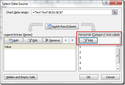
Guide: How to Name Column in Excel | Indeed.com Click "Modify" in the menu to access the Style dialog box. To launch the Format Cells dialog box, click the "Format" button in the dialog box. Click the "Font" tab in this second dialog box and select your desired font from the drop-down list. To close both dialog boxes and return to the worksheet, click "OK" twice. Use defined names to automatically update a chart range - Office Click the Design tab, click the Select Data in the Data group. Under Legend Entries (Series), click Edit. In the Series values box, type =Sheet1!Sales, and then click OK. Under Horizontal (Category) Axis Labels, click Edit. In the Axis label range box, type =Sheet1!Date, and then click OK. Microsoft Office Excel 2003 and earlier versions How to Move Excel Pivot Table Labels Quick Tricks Type the name of the label that you want to move Press Enter The existing labels shift down, and the moved label takes its new position. For example, type "West" in cell A4, over the existing District name, "Central" Then, press Enter, to complete the change. West moves to cell A4, and Central moves down to A5.

How to change data labels in excel 2013. How to Create and Customize a Treemap Chart in Microsoft Excel Select the data for the chart and head to the Insert tab. Click the "Hierarchy" drop-down arrow and select "Treemap." The chart will immediately display in your spreadsheet. And you can see how the rectangles are grouped within their categories along with how the sizes are determined. Show Changes and History of Edits in Excel - Excel Campus Viewing Changes. See the changes that have been made to a workbook by going to the Review tab. Then click the Show Changes button. This will open up a task pane on the right side of the worksheet that has a running list. The list contains all of the changes that have been made in the workbook. How to Create a Dynamic Chart Title in Excel Steps to Create Dynamic Chart Title in Excel Converting a normal chart title into a dynamic one is simple. But before that, you need a cell which you can link with the title. Here are the steps: Select chart title in your chart. Go to the formula bar and type =. Select the cell which you want to link with chart title. Hit enter. How to Change the X-Axis in Excel - Alphr Select Edit right below the Horizontal Axis Labels tab. Next, click on Select Range. Mark the cells in Excel, which you want to replace the values in the current X-axis of your graph. When you...

support.microsoft.com › en-us › officeChange the format of data labels in a chart To get there, after adding your data labels, select the data label to format, and then click Chart Elements > Data Labels > More Options. To go to the appropriate area, click one of the four icons ( Fill & Line , Effects , Size & Properties ( Layout & Properties in Outlook or Word), or Label Options ) shown here. Chart.ApplyDataLabels method (Excel) | Microsoft Docs Syntax expression. ApplyDataLabels ( Type, LegendKey, AutoText, HasLeaderLines, ShowSeriesName, ShowCategoryName, ShowValue, ShowPercentage, ShowBubbleSize, Separator) expression A variable that represents a Chart object. Parameters Example This example applies category labels to series one on Chart1. VB Copy Charts ("Chart1").SeriesCollection (1). How to Show Percentages in Stacked Column Chart in Excel? Implementation: Follow the below steps to show percentages in stacked column chart In Excel: Step 2: Select the entire data table. Step 3: To create a column chart in excel for your data table. Go to "Insert" >> "Column or Bar Chart" >> Select Stacked Column Chart. Step 4: Add Data labels to the chart. Goto "Chart Design" >> "Add ... Change the Font Size, Color, and Style of an Excel Form Control Label So to change the Label's formatting — even when it's linked to the same cell — you'll need to click the label, click the formula bar, and retype the cell link. Admittedly, everyone else might have already figured this one out. However, I'm still very excited.

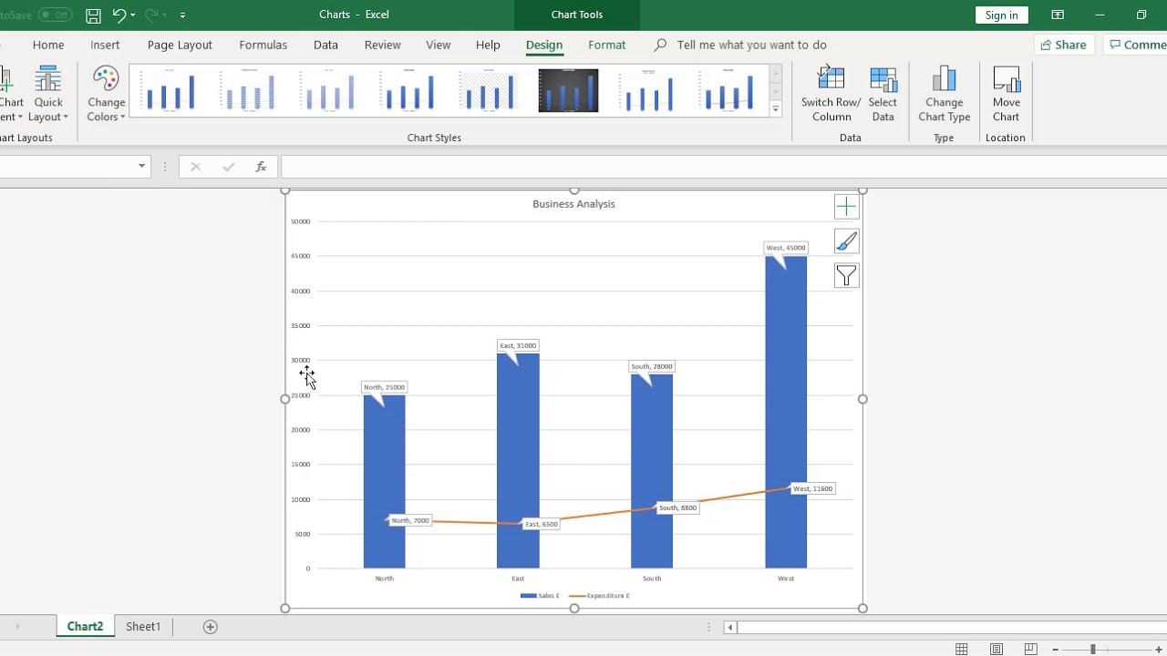
› charts › dynamic-chart-dataCreate Dynamic Chart Data Labels with Slicers - Excel Campus Feb 10, 2016 · Typically a chart will display data labels based on the underlying source data for the chart. In Excel 2013 a new feature called “Value from Cells” was introduced. This feature allows us to specify the a range that we want to use for the labels. Since our data labels will change between a currency ($) and percentage (%) formats, we need a ... mgconsulting.wordpress.com › 2013/12/09 › add-a-dataAdd a Data Callout Label to Charts in Excel 2013 Dec 09, 2013 · The new Data Callout Labels make it easier to show the details about the data series or its individual data points in a clear and easy to read format. How to Add a Data Callout Label. Click on the data series or chart. In the upper right corner, next to your chart, click the Chart Elements button (plus sign), and then click Data Labels. How to Change the Y Axis in Excel - Alphr Click the dropdown next to "Display Units," then make your selection such as "millions" or "hundreds." To label the displayed units, go to the "Axis Options -> Display units" section. Add a... Display data point labels outside a pie chart in a paginated report ... Create a pie chart and display the data labels. Open the Properties pane. On the design surface, click on the pie itself to display the Category properties in the Properties pane. Expand the CustomAttributes node. A list of attributes for the pie chart is displayed. Set the PieLabelStyle property to Outside. Set the PieLineColor property to Black.

Legends in Excel Charts - Formats, Size, Shape, and Position - Peltier Tech Blog

How to Sort by Ascending Order in Excel (3 Easy Methods) First, select the Range of Cells ( B5:C11) that you want to work with. Then, go to the Sort & Filter feature which you'll find in the Editing group under the Home tab. There, select the Sort A to Z option as we're sorting in Ascending Order. After selecting the option, you'll get your data organized based on Ascending Order of Employee Name.

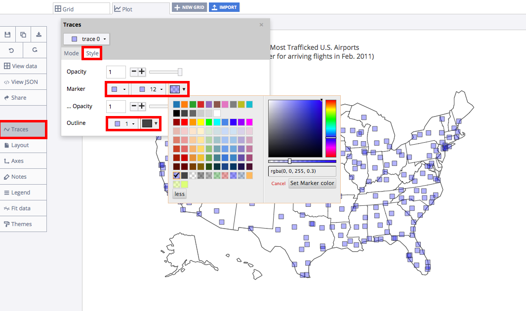
Make a Scatter Plot on a Map with Chart Studio and Excel

Excel Waterfall Chart: How to Create One That Doesn't Suck To create a waterfall chart in Excel 2013 and earlier, you had to define additional data series (with complicated formulas) in the data table and then make them invisible in the chart. And we're not talking about 1 invisible series. If the waterfall chart dipped below zero at one point, you needed at least seven additional series!

How to Add Data Labels to your Excel Chart in Excel 2013 - YouTube

How to Import Data From the Web Into Microsoft Excel Step 1: Launch Microsoft Excel on your computer. Step 2: On the Ribbon interface at the top, click on Data. Step 3: In the group titled Get & Transform Data, select From Web. Step 4: On the popup ...

How to Add Data Labels in Excel - Excelchat | Excelchat

chandoo.org › wp › change-data-labels-in-chartsHow to Change Excel Chart Data Labels to Custom Values? May 05, 2010 · Now, click on any data label. This will select “all” data labels. Now click once again. At this point excel will select only one data label. Go to Formula bar, press = and point to the cell where the data label for that chart data point is defined. Repeat the process for all other data labels, one after another. See the screencast.

Advanced Graphs Using Excel : 3D-histogram in Excel

Excel IF function with multiple conditions - Ablebits.com The generic formula of Excel IF with two or more conditions is this: IF (AND ( condition1, condition2, …), value_if_true, value_if_false) Translated into a human language, the formula says: If condition 1 is true AND condition 2 is true, return value_if_true; else return value_if_false. Suppose you have a table listing the scores of two tests ...

Show Trend Arrows in Excel Chart Data Labels | Excel, Chart, Excel tutorials

How to Make a Pie Chart in Excel (Only Guide You Need) To do this select the More Options from Data labels under the Chart Elements or by selecting the chart right click on to the mouse button and select Format Data Labels. This will open up the Format Data Label option on the right side of your worksheet. Click on the percentage. If you want the value with the percentage click on both and close it.

How to Print Labels from Excel

› excel › how-to-add-total-dataHow to Add Total Data Labels to the Excel Stacked Bar Chart Apr 03, 2013 · Step 4: Right click your new line chart and select “Add Data Labels” Step 5: Right click your new data labels and format them so that their label position is “Above”; also make the labels bold and increase the font size. Step 6: Right click the line, select “Format Data Series”; in the Line Color menu, select “No line”

Fixing Your Excel Chart When the Multi-Level Category Label Option is Missing. - Excel Dashboard ...

How To Summarize Data in Excel: Top 10 Ways - ExcelChamp Calculate SUM: Click on the Autosum icon on the Home tab of Microsoft Office to activate the Sum function of Excel. Then select the data range of the column you want to summarize. Here's an example: Calculate COUNT: Click on the drop-down icon on the Autosum button on the Home tab of Microsoft Excel.

Format Number Options for Chart Data Labels in Excel 2011 for Mac

How to mail merge and print labels from Excel - Ablebits If the Use the current document option is inactive, then select Change document layout, click the Label options… link, and then specify the label information. Configure label options. Before proceeding to the next step, Word will prompt you to select Label Options such as: Printer information - specify the printer type.

How To Add Data Labels To A Chart in Microsoft Excel - YouTube

Position labels in a paginated report chart - Microsoft Report Builder ... On the design surface, right-click the chart and select Show Data Labels. Open the Properties pane. On the View tab, click Properties On the design surface, click the series. The properties for the series are displayed in the Properties pane. In the Data section, expand the DataPoint node, then expand the Label node.

Top 24 Weird Invention In Japan: How do change the default Excel spreadsheet download setting in ...

Unlink Chart Data - Peltier Tech If the chart links to data in a closed Excel workbook, the SERIES formula includes the path, then the workbook name in square brackets, and finally the worksheet name. ... elements (rescale the axes, change marker styles or colors, etc.). Therefore, this method is unsuitable for use within Excel. Change the Cell References to Hard-Coded Values ...

microsoft excel - Adding data label only to the last value - Super User

Format Chart Axis in Excel - Axis Options Analyzing Format Axis Pane. Right-click on the Vertical Axis of this chart and select the "Format Axis" option from the shortcut menu. This will open up the format axis pane at the right of your excel interface. Thereafter, Axis options and Text options are the two sub panes of the format axis pane.

excel - How do I update the data label of a chart? - Stack Overflow

Excel Pivot Table Field Layout Changes and Macro Samples To change the data to a vertical layout, drag the Values button in the Pivot Table Field List, from the Column Labels area to the Row Labels area. In most cases, the Values button should be positioned below the other fields in the Row Labels area. After you move the Values label to the Row Labels area, the data fields will be arranged vertically.

Excel chart type: How to create a variety of chart types

support.microsoft.com › en-us › officeEdit titles or data labels in a chart - support.microsoft.com Change the position of data labels. You can change the position of a single data label by dragging it. You can also place data labels in a standard position relative to their data markers. Depending on the chart type, you can choose from a variety of positioning options. On a chart, do one of the following:

Waterfall Chart - Page 2 of 2 - Beat Excel!

How to Change Commas to Decimal Points and Vice Versa in Excel (5 Ways) To change commas to decimals using Replace: Select the range of cells in which you want to replace commas with decimals. You may select a range of cells, a column or columns or the entire worksheet. Press Ctrl + 1 or right-click and select Format Cells. A dialog box appears.

How to Create a Chart in Microsoft Excel - Tech Support

Custom Excel number format - Ablebits.com To create a custom Excel format, open the workbook in which you want to apply and store your format, and follow these steps: Select a cell for which you want to create custom formatting, and press Ctrl+1 to open the Format Cells dialog. Under Category, select Custom. Type the format code in the Type box. Click OK to save the newly created format.

Excel Spreadsheets Help: How to Combine Excel Files

How to Print Labels from Excel - Lifewire Choose Start Mail Merge > Labels . Choose the brand in the Label Vendors box and then choose the product number, which is listed on the label package. You can also select New Label if you want to enter custom label dimensions. Click OK when you are ready to proceed. Connect the Worksheet to the Labels

Share :