38 how to add percentage and category name data labels in excel

How to add data labels from different column in an Excel chart? Right click the data series in the chart, and select Add Data Labels > Add Data Labels from the context menu to add data labels. 2. Click any data label to select all data labels, and then click the specified data label to select it only in the chart. 3. Excel tutorial: How to use data labels When you check the box, you'll see data labels appear in the chart. If you have more than one data series, you can select a series first, then turn on data labels for that series only. You can even select a single bar, and show just one data label. In a bar or column chart, data labels will first appear outside the bar end.

Format Data Labels in Excel- Instructions - TeachUcomp, Inc. To do this, click the "Format" tab within the "Chart Tools" contextual tab in the Ribbon. Then select the data labels to format from the "Chart Elements" drop-down in the "Current Selection" button group. Then click the "Format Selection" button that appears below the drop-down menu in the same area.

How to add percentage and category name data labels in excel

Add or remove data labels in a chart - support.microsoft.com Add data labels to a chart Click the data series or chart. To label one data point, after clicking the series, click that data point. In the upper right corner, next to the chart, click Add Chart Element > Data Labels. To change the location, click the arrow, and choose an option. Multiple data labels (in separate locations on chart) Running Excel 2010 2D pie chart I currently have a pie chart that has one data label already set. The Pie chart has the name of the category and value as data labels on the outside of the graph. I now need to add the percentage of the section on the INSIDE of the graph, centered within the pie section. Custom Chart Data Labels In Excel With Formulas Follow the steps below to create the custom data labels. Select the chart label you want to change. In the formula-bar hit = (equals), select the cell reference containing your chart label's data. In this case, the first label is in cell E2. Finally, repeat for all your chart laebls.

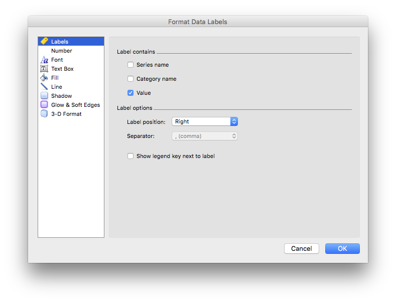
How to add percentage and category name data labels in excel. How to show data label in "percentage" instead of - Microsoft Community Select Format Data Labels Select Number in the left column Select Percentage in the popup options In the Format code field set the number of decimal places required and click Add. (Or if the table data in in percentage format then you can select Link to source.) Click OK Regards, OssieMac Report abuse 8 people found this reply helpful · Understanding Excel Chart Data Series, Data Points, and Data Labels Series Names: Identifies the columns or rows of chart data in the worksheet. Series names are commonly used for column charts, bar charts, and line graphs. Category Names: Identifies the individual data points in a single series of data. These are commonly used for pie charts. Percentage Labels: Calculated by dividing the individual fields in a ... Free Budget vs. Actual chart Excel Template - Download 16.05.2018 · Create Budget vs Actual chart with smart labels in Excel – Tutorial. If you are in a hurry to make such a chart, download the template, plug in your values and you are good to go. For instructions on how to create them in Excel, read along. Step 1: Getting the data. Set up your data. Let’s say you have budgets and actual values for a bunch ... Excel for Commerce | Analyze large data sets in Excel 07.05.2015 · There are professional data analysts out there who tackle “big data” with complex software, but it’s possible to do a surprising amount of analysis with Microsoft Excel. In this case, we’re using baby names from California based on the United States Social Security Baby Names Database. In this tutorial, you’ll not only learn how to manipulate big data in Excel, you’ll learn …

Change the format of data labels in a chart To get there, after adding your data labels, select the data label to format, and then click Chart Elements > Data Labels > More Options. To go to the appropriate area, click one of the four icons ( Fill & Line, Effects, Size & Properties ( Layout & Properties in Outlook or Word), or Label Options) shown here. How to use Excel Data Model & Relationships » Chandoo.org - Learn Excel ... 01.07.2013 · Things to keep in mind when you using relationships. Same data types in both columns: Columns that you are connecting in both tables should have same data type (ie both numbers or dates or text etc.) One to one or One to many relationships only: Excel 2013 supports only one to many or one to one relationships.That means one of the tables must have no … Pivot Chart Data Label Help Needed - Microsoft Community Open the Excel file with Pivot Chart and enabled with Data Labels> Click on the Labels displayed in the Chart> Right-click> Click Format Data Labels> Label Options> Number> In the Category, select the format as per your requirement. Here is the reference article: Change the format of data labels in a chart. Solved: change data label to percentage - Power BI Hi @MARCreading. pick your column in the Right pane, go to Column tools Ribbon and press Percentage button. do not hesitate to give a kudo to useful posts and mark solutions as solution. LinkedIn. Message 2 of 7. 1,596 Views. 1.

excel - How can I add chart data labels with percentage? - Stack Overflow I want to add chart data labels with percentage by default with Excel VBA. Here is my code for creating the chart: Private Sub CommandButton2_Click() ActiveSheet.Shapes.AddChart.Select ActiveChart. How to show values in data labels of Excel ... - MrExcel Message Board 2) Move Value data series to 2nd Axis 3) Change Value data series Fill from Automatic to No Fill 4) Change 2nd Vertical Axis Labels to None 5) Add Data Labels to Value data series Hope this helps. Steve=True D dendres New Member Joined Aug 1, 2015 Messages 14 Aug 3, 2015 #3 Hi Steve=True, Thank you for the help. Error Bars in Excel (Examples) | How To Add Excel Error Bar? This website or its third-party tools use cookies, which are necessary to its functioning and required to achieve the purposes illustrated in the cookie policy. How to create a chart with both percentage and value in Excel? In the Format Data Labels pane, please check Category Name option, and uncheck Value option from the Label Options, and then, you will get all percentages and values are displayed in the chart, see screenshot: 15.

Working with Charts — XlsxWriter Documentation

How to Customize Your Excel Pivot Chart Data Labels - dummies To add data labels, just select the command that corresponds to the location you want. To remove the labels, select the None command. If you want to specify what Excel should use for the data label, choose the More Data Labels Options command from the Data Labels menu. Excel displays the Format Data Labels pane.

How to Create a Pie Chart in Excel | Smartsheet

The Chart Class — XlsxWriter Documentation categories: This sets the chart category labels. The category is more or less the same as the X axis. In most chart types the categories property is optional and the chart will just assume a sequential series from 1..n. name: Set the name for the series. The name is displayed in the formula bar. For non-Pie/Doughnut charts it is also displayed ...

Excel & Google Sheets Chart Resources That Will Make Your Life Easier | PPC Hero

How To Add and Remove Legends In Excel Chart? - EDUCBA Excel Data Analysis Training (15 Courses, 8+ Projects) Excel for Marketing Training (8 Courses, 13+ Projects) ... If we want to add the legend in the excel chart, it is a quite similar way how we remove the legend in the same way. Select the chart and click on the “+” symbol at the top right corner. From the pop-up menu, give a tick mark to the Legend. Now Legend is available again. …

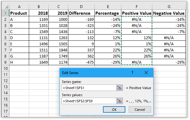
Quickly create a positive negative bar chart in Excel

Chart.ApplyDataLabels method (Excel) | Microsoft Docs For the Chart and Series objects, True if the series has leader lines. Pass a Boolean value to enable or disable the series name for the data label. Pass a Boolean value to enable or disable the category name for the data label. Pass a Boolean value to enable or disable the value for the data label.

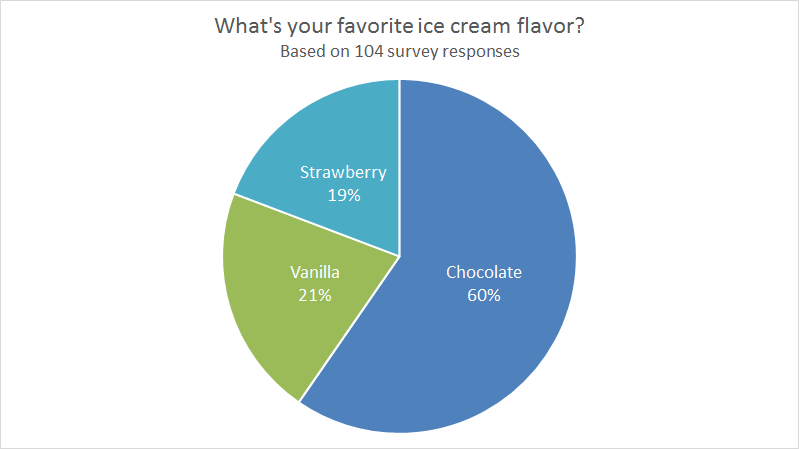
Pie Chart: Survey results favorite ice cream flavor | Exceljet

How to show percentage in Excel - Ablebits To do this, open the Format Cells dialog either by pressing Ctrl + 1 or right-clicking the cell and selecting Format Cells… from the context menu. Make sure the Percentage category is selected and specify the desired number of decimal places in the Decimal places box. When done, click the OK button to save your settings.

Business Diary: October 2011

How to show data labels in PowerPoint and place them ... - think-cell To reset a label and (re-)insert text fields, use the label content control (Label content) or simply click on the exclamation mark, if there is one. Note: Due to a limitation in Excel only the first 255 characters of text in a datasheet cell will be displayed in a label in PowerPoint.

Learn SEO The Ultimate Guide For SEO Beginners 2020 - Your Optimized Solutions

How to Change Excel Chart Data Labels to Custom Values? Now, click on any data label. This will select "all" data labels. Now click once again. At this point excel will select only one data label. Go to Formula bar, press = and point to the cell where the data label for that chart data point is defined. Repeat the process for all other data labels, one after another. See the screencast. Points to note:

Pie Charts bring in Best Presentation for Growth

Best Types of Charts in Excel for Data Analysis ... - Optimize Smart 29.04.2022 · Use the moving average trendline if there is a lot of fluctuation in your data. How to add a chart to an Excel spreadsheet? To add a chart to an Excel spreadsheet, follow the steps below: Step-1: Open MS Excel and navigate to the spreadsheet, which contains the data table you want to use for creating a chart. Step-2: Select data for the chart:

Share :