45 chart data labels excel

How to create Custom Data Labels in Excel Charts Create the chart as usual. Add default data labels. Click on each unwanted label (using slow double click) and delete it. Select each item where you want the custom label one at a time. Press F2 to move focus to the Formula editing box. Type the equal to sign. Now click on the cell which contains the appropriate label. Excel.ChartDataLabels class - Office Add-ins | Microsoft Docs The request context associated with the object. This connects the add-in's process to the Office host application's process. Specifies the format of chart data labels, which includes fill and font formatting. Specifies the horizontal alignment for chart data label. See Excel.ChartTextHorizontalAlignment for details.

› charts › dynamic-chart-dataCreate Dynamic Chart Data Labels with Slicers - Excel Campus Feb 10, 2016 · Typically a chart will display data labels based on the underlying source data for the chart. In Excel 2013 a new feature called “Value from Cells” was introduced. This feature allows us to specify the a range that we want to use for the labels. Since our data labels will change between a currency ($) and percentage (%) formats, we need a ...

Chart data labels excel

support.microsoft.com › en-us › officeEdit titles or data labels in a chart - support.microsoft.com On a chart, click one time or two times on the data label that you want to link to a corresponding worksheet cell. The first click selects the data labels for the whole data series, and the second click selects the individual data label. Right-click the data label, and then click Format Data Label or Format Data Labels. Adding rich data labels to charts in Excel 2013 - Microsoft 365 Blog One familiar and simple way is just single click on any data value (or column, in this example) to select the entire data series that it belongs to. Above, I have clicked all of the blue columns. Once the series is selected, I can right-click any column to pull up the context menu, then click the Add Data Labels entry. › excel › how-to-add-total-dataHow to Add Total Data Labels to the Excel Stacked Bar Chart Apr 03, 2013 · Step 4: Right click your new line chart and select “Add Data Labels” Step 5: Right click your new data labels and format them so that their label position is “Above”; also make the labels bold and increase the font size. Step 6: Right click the line, select “Format Data Series”; in the Line Color menu, select “No line” Step 7 ...

Chart data labels excel. How To Use Dynamic Data Labels To Create Interactive Excel Charts To create a column chart with dynamic data labels, you need to follow these given steps. Select the data & Create a Combo Chart. Now select the column chart for revenue data and a line chart with marker for data labels. Add Data Labels to the Line Chart With Marker. After then remove the Line Color and Marker Color. Adding Data Labels to Your Chart (Microsoft Excel) To add data labels in Excel 2013 or Excel 2016, follow these steps: Activate the chart by clicking on it, if necessary. Make sure the Design tab of the ribbon is displayed. (This will appear when the chart is selected.) Click the Add Chart Element drop-down list. Select the Data Labels tool. excel - Positioning of Datalabels in a chart - Stack Overflow Show activity on this post. I'm trying to positioning the labels of two series in a combo chart. I first position all the series using xlLabelPositionAbove and xlLabelPositionOutsideEnd and then I modify each label point by point. The problem is that if I break the code before the For next loop, the routine has the time to make the first ... Excel Charts - Aesthetic Data Labels - Tutorialspoint To place the data labels in the chart, follow the steps given below. Step 1 − Click the chart and then click chart elements. Step 2 − Select Data Labels. Click to see the options available for placing the data labels. Step 3 − Click Center to place the data labels at the center of the bubbles. Format a Single Data Label

How do I replicate an Excel chart but change the data? Oct 18, 2018 · To update the data range, double click on the chart, and choose Change Date Range from the Mekko Graphics ribbon. Select your new data range and click OK in the floating Chart Data dialog box. Your data can be in the same worksheet as the chart, as shown in the example below, or in a different worksheet. Add a DATA LABEL to ONE POINT on a chart in Excel Steps shown in the video above: Click on the chart line to add the data point to. All the data points will be highlighted. Click again on the single point that you want to add a data label to. Right-click and select ' Add data label ' This is the key step! Right-click again on the data point itself (not the label) and select ' Format data label '. Format Data Labels in Excel- Instructions - TeachUcomp, Inc. To do this, click the "Format" tab within the "Chart Tools" contextual tab in the Ribbon. Then select the data labels to format from the "Chart Elements" drop-down in the "Current Selection" button group. Then click the "Format Selection" button that appears below the drop-down menu in the same area. chandoo.org › wp › change-data-labels-in-chartsHow to Change Excel Chart Data Labels to Custom Values? May 05, 2010 · Now, click on any data label. This will select “all” data labels. Now click once again. At this point excel will select only one data label. Go to Formula bar, press = and point to the cell where the data label for that chart data point is defined. Repeat the process for all other data labels, one after another. See the screencast.

How to hide zero data labels in chart in Excel? - ExtendOffice If you want to hide zero data labels in chart, please do as follow: 1. Right click at one of the data labels, and select Format Data Labels from the context menu. See screenshot: 2. In the Format Data Labels dialog, Click Number in left pane, then select Custom from the Category list box, and type #"" into the Format Code text box, and click Add button to add it to Type list box. Custom Data Labels with Colors and Symbols in Excel Charts - [How To] Step 4: Select the data in column C and hit Ctrl+1 to invoke format cell dialogue box. From left click custom and have your cursor in the type field and follow these steps: Press and Hold ALT key on the keyboard and on the Numpad hit 3 and 0 keys. Let go the ALT key and you will see that upward arrow is inserted. Chart.ApplyDataLabels method (Excel) | Microsoft Docs For the Chart and Series objects, True if the series has leader lines. Pass a Boolean value to enable or disable the series name for the data label. Pass a Boolean value to enable or disable the category name for the data label. Pass a Boolean value to enable or disable the value for the data label. How to add or move data labels in Excel chart? In Excel 2013 or 2016. 1. Click the chart to show the Chart Elements button . 2. Then click the Chart Elements, and check Data Labels, then you can click the arrow to choose an option about the data labels in the sub menu. See screenshot: In Excel 2010 or 2007. 1. click on the chart to show the Layout tab in the Chart Tools group. See ...

10 ways to present variance analysis reports in Excel - PakAccountants.com

Excel.ChartDataLabel class - Office Add-ins | Microsoft Docs Represents the distance, in points, from the top edge of chart data label to the top of chart area. Value is null if the chart data label is not visible. vertical Alignment: Represents the vertical alignment of chart data label. See Excel.ChartTextVerticalAlignment for details. This property is valid only when TextOrientation of data label is 0.

How to Create a Geographical Map Chart in Microsoft Excel

support.microsoft.com › en-us › officeAdd or remove data labels in a chart - support.microsoft.com Click the data series or chart. To label one data point, after clicking the series, click that data point. In the upper right corner, next to the chart, click Add Chart Element > Data Labels. To change the location, click the arrow, and choose an option. If you want to show your data label inside a text bubble shape, click Data Callout.

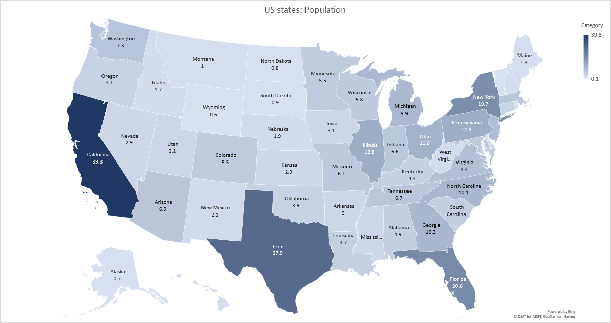
Excel map chart

Change the format of data labels in a chart To get there, after adding your data labels, select the data label to format, and then click Chart Elements > Data Labels > More Options. To go to the appropriate area, click one of the four icons ( Fill & Line, Effects, Size & Properties ( Layout & Properties in Outlook or Word), or Label Options) shown here.

Creating Pie Chart and Adding/Formatting Data Labels (Excel) - YouTube

› make-chart-x-axis-labelsMake Chart X Axis Labels Display below Negative Data - Excel How Aug 21, 2018 · Move X Axis to Bottom for Negative Data. When you created a bar chart or line chart in your worksheet, and the X Axis labels are stuck at 0 position of the Axis. And if you source data have negative values, and you want to move X Axis labels below negative, how to achieve it.

Basic Excel Chart Formatting - MS Excel Charting Tutorial Part 4 | Vertical Horizons

Add / Move Data Labels in Charts - Excel & Google Sheets We'll start with the same dataset that we went over in Excel to review how to add and move data labels to charts. Add and Move Data Labels in Google Sheets Double Click Chart Select Customize under Chart Editor Select Series 4. Check Data Labels 5. Select which Position to move the data labels in comparison to the bars.

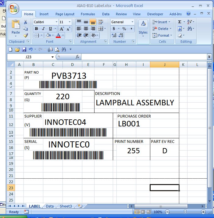
Label Template Excel | printable label templates

Excel tutorial: How to use data labels Generally, the easiest way to show data labels to use the chart elements menu. When you check the box, you'll see data labels appear in the chart. If you have more than one data series, you can select a series first, then turn on data labels for that series only. You can even select a single bar, and show just one data label.

How to Make Charts and Graphs in Excel | Smartsheet

› documents › excelHow to add data labels from different column in an Excel chart? Right click the data series in the chart, and select Add Data Labels > Add Data Labels from the context menu to add data labels. 2. Click any data label to select all data labels, and then click the specified data label to select it only in the chart. 3.

Custom Data Labels with Colors and Symbols in Excel Charts - [How To] - PakAccountants.com

Use a screen reader to add a title, data labels, and a legend to a ... Select the chart that you want to work with. To open the Add Chart Element menu, press Alt+J, C, A. To add data callout labels to the chart, press D and then U. Tip: To remove data labels, select the chart, and then press Alt+J, C, A, D, and then N. Add a legend to a chart Legends help you to quickly understand data relationships in a chart.

How to Change Excel Chart Data Labels to Custom Values?

Plot Multiple Data Sets on the Same Chart in Excel Jun 29, 2021 · The present y-axis line is having much higher values and the percentage line will be having values lesser than 1 i.e. in decimal values. Hence, we need a secondary axis in order to plot the two lines in the same chart. In Excel, it is also known as clustering of two charts. The steps to add a secondary axis are as follows : 1. Open

Show Trend Arrows in Excel Chart Data Labels

Create a multi-level category chart in Excel - ExtendOffice Select the dots, click the Chart Elements button, and then check the Data Labels box. 23. Right click the data labels and select Format Data Labels from the right-clicking menu. 24. In the Format Data Labels pane, please do as follows. 24.1) Check the Value From Cells box;

Custom Data Labels with Colors and Symbols in Excel Charts – [How To] - KING OF EXCEL

Custom Chart Data Labels In Excel With Formulas Follow the steps below to create the custom data labels. Select the chart label you want to change. In the formula-bar hit = (equals), select the cell reference containing your chart label's data. In this case, the first label is in cell E2. Finally, repeat for all your chart laebls.

How-to Use Data Labels from a Range in an Excel Chart - Excel Dashboard Templates

How to Use Cell Values for Excel Chart Labels Select the chart, choose the "Chart Elements" option, click the "Data Labels" arrow, and then "More Options." Uncheck the "Value" box and check the "Value From Cells" box. Select cells C2:C6 to use for the data label range and then click the "OK" button. The values from these cells are now used for the chart data labels.

How-to Use Data Labels from a Range in an Excel Chart - Excel Dashboard Templates

How to add total labels to stacked column chart in Excel? Add total labels to stacked column chart in Excel Supposing you have the following table data. 1. Firstly, you can create a stacked column chart by selecting the data that you want to create a chart, and clicking Insert > Column, under 2-D Column to choose the stacked column. See screenshots: And now a stacked column chart has been built. 2.

Do My Excel Blog: How to design a multiple clustered bar chart series in Excel

How to I rotate data labels on a column chart so that they are ... To change the text direction, first of all, please double click on the data label and make sure the data are selected (with a box surrounded like following image). Then on your right panel, the Format Data Labels panel should be opened. Go to Text Options > Text Box > Text direction > Rotate

Share :